Algorithm Summarize: Advanced Motion Planning and AI
Table of Contents
- Lattice Planning
- MPPI (Model Predictive Path Integral Control)
- AlphaGo, AlphaZero, and Monte-Carlo Tree Search
Lattice Planning
Introduction
Lattice planning is a technique in robotics and motion planning that discretizes the continuous environment into a grid-like structure, known as a lattice. It enables the efficient computation of paths and motions by representing the search space as a set of states connected through predefined actions.
This approach simplifies planning by converting complex, continuous problems into simpler, discrete ones, allowing algorithms like A* or D* to find optimal or near-optimal paths. Lattice planning is particularly useful for robot navigation in structured environments where obstacles and constraints can be effectively represented in a grid.
Principles
Lattice Construction

Key Components:
- Motion primitives: These are small, simple movements that the robot can make, such as moving forward by a fixed amount or turning a fixed angle. These primitive movements are predefined, allowing the robot to use them without recalculating the entire path every time.
- Collision checking: During pre-computation, we need to verify whether each potential motion (or trajectory) within the lattice is collision-free (physically feasible). If a transition leads to a collision, that path is removed from the lattice.
Path Searching
The state lattice is specified by a regular sampling of nodes in the state space and edges between them. Edges correspond to feasible and local paths between nodes (also called motion primitives or control set). Since the state lattice is a directed graph, any graph search algorithm is appropriate for finding a path in it.
Algorithm: A (or D for dynamic updates)**
- Heuristic: typically Euclidean distance in (𝑥,𝑦) or a precomputed 2D cost‐to‐go lookup
- Heuristic search is a problem-solving technique that uses a heuristic function to guide the search process toward the goal efficiently. A heuristic is an estimate of the cost or distance from a current state to the goal state.
- It helps prioritize which states to explore first in the search space, aiming to find a solution more quickly than by exploring all possibilities equally.
Guarantees:
- Resolution completeness (finds a path if one exists at the chosen discretization)
- Near-optimality (with an admissible heuristic and fixed primitive set)
A* Algorithm
The A* Algorithm is widely used for lattice-based path planning because it's both efficient and guarantees finding the shortest path. Here's how it works:
- A* searches the graph (the lattice) by looking at the state space and considering both the cost to get to a state (e.g., time, energy, distance) and an estimate of how far the goal is from the current state (heuristic).
- It keeps expanding the nodes (states) that seem to be the most promising (those with the lowest total cost), until it reaches the goal.
Dynamic Replanning
When encountering obstacles or sudden change in traffic, the robot needs to react. It needs to update the motion primitives. Rather than recalculating the whole route, lattice planning saves time by only considering the blocked motion primitives (future routes). In this case, algorithms specifically designed by dynamic planning are used (D* Lite, etc.)
MPPI (Model Predictive Path Integral Control)
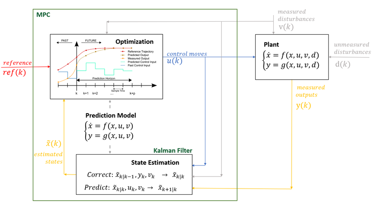
Model Predictive Control (MPC)
At each time step, you (virtually) simulate "what happens next" over a finite horizon, pick the best action sequence according to some cost function, then apply only the first action and repeat at the next step.
You basically predict the sequence and predict the cost and chose the one with the lowest cost:
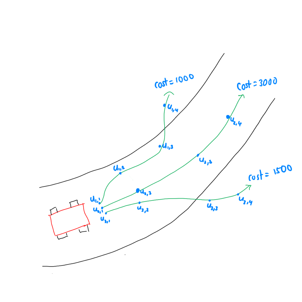
MPPI Algorithm
- Start with a control sequence (either zero or heuristic guess)
- Add noise (e.g. Gaussian) and generate perturbed paths
- Roll out dynamics: predict and calculate the costs of the perturbed paths
Cost Function:
The cost function includes:
- State cost and control cost
- Terminal cost at the end of the horizon
- is the desired state
- and are weighting matrices
- Assign weight: paths with lower costs have higher weight
Trajectory Costs:
Minimum Cost:
Importance Weight:
where () is a temperature parameter.
Normalized Weight:
Optimal Control:
Implementation
Control Update Visualization:
Results:
![]()
Example Code
def _compute_weights(self, S: np.ndarray) -> np.ndarray:
    """compute weights for each sample"""
    # prepare buffer
    w = np.zeros((self.K))
    # calculate rho
    rho = S.min()
    # calculate eta
    eta = 0.0
    for k in range(self.K):
        eta += np.exp( (-1.0/self.param_lambda) * (S[k]-rho) )
    # calculate weight
    for k in range(self.K):
        w[k] = (1.0 / eta) * np.exp( (-1.0/self.param_lambda) * (S[k]-rho) )
    '''Standardization, let the weights sum up to 1'''
    return w

# Update control sequence
w = self._compute_weights(S)
# calculate w_k * epsilon_k
w_epsilon = np.zeros((self.T, self.dim_u))
for t in range(0, self.T): # loop for time step t = 0 ~ T-1
    for k in range(self.K):
        w_epsilon[t] += w[k] * epsilon[k, t]

# Smooth control sequence with moving average
w_epsilon = self._moving_average_filter(w_epsilon, window_size=10)
Why MPPI over MPC
MPC can be stuck in local solutions as it is ==gradient based==. Imagine on a hilly terrain and you are trying to find the lowest valley - you may only find the local minimum as you can't see other low valleys. MPPI solves this better as it does not try to find a solution, but instead tests out different paths and calculates their costs.
Key Advantages:
- Nonconvex means the problem has many local solutions, and it's hard to find the best one.
- Gradient-based methods like MCP may get stuck in suboptimal solutions (local minima).
- MPPI explores multiple paths and can "discover" better solutions by avoiding being stuck in local minima.
AlphaGo, AlphaZero, and Monte-Carlo Tree Search
Reinforcement Learning
Key concepts in reinforcement learning:
- Exploration: searching for new strategies
- Exploitation: utilizing the found best solution so far
- State Value: specifies how good it is for an agent to be in a particular state with a policy
A good state should:
- Explore all potential options at the time
- Quickly identify the best one
- Keep looking for other good options whilst validating how good the current best is
- Improve the longer it has to think about it
Monte Carlo Tree Search
Monte Carlo Tree Search (MCTS) is a heuristic search algorithm that has gained significant attention in artificial intelligence, especially in decision-making and game playing. It effectively handles complex and strategic scenarios with large search spaces, where traditional algorithms might struggle.
Overview
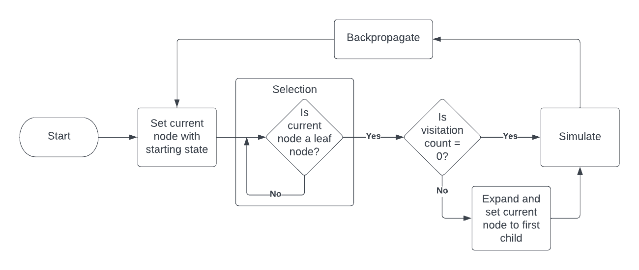
| Phase | What happens | Why it matters |
|---|---|---|
| Selection | Starting at the root (current position), walk down the tree by repeatedly choosing a child node using a selection policy (most commonly UCB). | Balances exploitation (using what we already know) and exploration (trying unfamiliar moves). |
| Expansion | When you reach a leaf that is not terminal and still has unexplored actions, create one or more child nodes for those actions. | Grows the search frontier only where needed, keeping the tree sparse. |
| Simulation | From the newly added node, play out a playout policy (often uniform-random) until a terminal state. | Provides a cheap estimate of the value of that move without exhaustive search. |
| Backpropagation | Propagate the simulation's result back up the path, updating visit counts and total reward for each node. | Makes future selections smarter by incorporating new knowledge. |
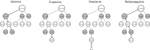
Selection
Upper Confidence Bound (UCB) Formula:
Where:
- : total reward of node (number of wins)
- : number of visits to node
- : visits to the parent
- : exploration constant (commonly , tunable)
The formula balances:
- (win rate) - higher win rate leads to higher UCB (exploitation)
- - decreases as a route is chosen more often, encouraging exploration
- - determines the weight of exploration vs exploitation
Expansion and Simulation
When a node has been visited, we:
- Make it the parent node
- Add its children nodes
- Simulate from the selected child node with random choices
- Assign outcomes:
Win = +1Lose = -1Draw = 0
Backpropagation
In this phase, we backpropagate and update results through the tree:
- Start from the simulated leaf node
- Update all nodes in the path back to root
- Update visit counts and rewards
- Use these updates to inform future selection
Advantages of MCTS
-
Domain Agnostic
- Works without special domain knowledge
- Applies to many tasks through simulation and statistics
- No need for custom rules or models
-
Interruptible
- Can stop at any time
- Always provides the best move found so far
- Useful for real-time scenarios
-
Efficient Search
- Grows asymmetrically towards promising areas
- Focuses computation where most useful
- Improves efficiency and decision quality
AlphaZero
AlphaZero combines three key components:
-
Value Network
- Outputs win probability
- Eliminates need for expensive rollouts
- Guides search efficiently
-
Policy Network
- Enables heuristic search
- Excludes unlikely moves
- Improves search efficiency
-
Monte Carlo Tree Search
- Can be interrupted anytime
- Provides best current answer
- Combines with neural networks
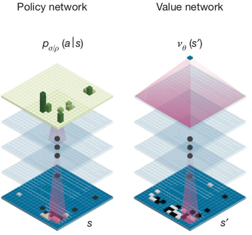
Neural Networks in AlphaZero
Value Network
The value network:
- Takes board state as input
- Outputs win probability (-1 to +1)
- Uses ResNet-style architecture
- Trained on self-play data
Training process:
- Collect game states and outcomes
- Train network to predict game results
- Continuously improve through self-play
- Guide MCTS with learned values
Policy Network
Training happens in two phases:
-
Supervised Learning (SL):
Loss_SL = -∑_a p_true(a|s) log p_θ(a|s)- Learn from human expert moves
- Mimic strong play patterns
- Build initial strategy
-
Reinforcement Learning (RL):
Loss_RL = -E_π[log p_θ(a|s) · R]- Self-play improvement
- Win = +1, Loss = -1
- Maximize winning probability
Softmax in Policy Networks
The policy network uses softmax to convert logits to probabilities:
Benefits:
- Fast computation
- Natural probability distribution
- Enables both exploration and exploitation
Note: The policy network is preferred for move selection because:
- It's faster (softmax computation)
- Trained on human expertise first
- Refined through self-play