Dynamic Window Approach (DWA) Planner

The Dynamic Window Approach (DWA) is a real-time local planner that generates feasible paths for a robot while considering its dynamics. It focuses on planning only for a very short period and aims for faster response time.

DWA Planner

What is the "Dynamic Window"?

In order to consider the limited accelerations by the robot's motors, the overall search space is reduced to the dynamic window, which contains only the velocities that can be reached within the next time interval.

1. Searching Space

Generating Circular Trajectories: Circular trajectories are generated, uniquely determined by the pairs (v, ω) of translational and rotational velocities.
Choosing Admissible Velocities: A velocity is considered admissible if the robot can stop before it reaches an obstacle.
Creating a Dynamic Window: This step restricts the admissible velocities to those that can be reached within a short time interval, given the limited accelerations of the robot.

2. Optimization

The optimization process uses an objective function for evaluation:

$G(v, ω) = \sigma(\alpha \cdot \text{heading}(v, ω) + \beta \cdot \text{dist}(v, ω) + \gamma \cdot \text{vel}(v, ω))$

Where:

Target Heading: Heading measures progress towards the goal. It is maximized when the robot moves directly towards the target.
Distance: Distance measures the closeness to the nearest obstacle. Smaller distances are preferred.
Velocity: The forward velocity, with higher values enabling faster movements.

3 Key Questions

"Where can I go?": This question is answered by calculating all possible velocities (linear and angular) that the robot can achieve in the next short moment, considering its current speed and acceleration limits. The set of achievable velocities forms the Dynamic Window.
"What would happen if I went there?": For each possible velocity pair (linear speed and angular speed), the algorithm simulates a short trajectory. The goal is to evaluate how well each velocity achieves the desired progress while avoiding obstacles.
"Which of these options is the best?": The algorithm "scores" each hypothetical trajectory using the objective function. This function evaluates three priorities:
- Goal Heading: Progress towards the goal.
- Obstacle Clearance: Distance from obstacles.
- Velocity: Speed of movement.

Constraints

The dynamic window is determined by two main constraints:

Robot's Absolute Limits:
- The robot cannot exceed its maximum speed or yaw rate.
- Linear velocities ( $v$ ) are restricted to the range [min_speed, max_speed].
- Angular velocities ( $w$ ) are restricted to [max_yaw_rate, -max_yaw_rate].
Acceleration Limits:
- The robot can only change velocity within the limits of its acceleration. The velocity can change by a maximum of max_accel * dt in the next time step.
- Linear velocities ( $v$ ) are updated as:
  $v_{\text{new}} = v_{\text{current}} + \text{max\_accel} \cdot dt$
- Angular velocities ( $w$ ) are updated as:
  $w_{\text{new}} = w_{\text{current}} + \text{max\_delta\_yaw\_rate} \cdot dt$

Dynamic Window

The Dynamic Window is the intersection of the robot's velocity limits and acceleration constraints. It defines the set of velocities that are both possible and achievable at a given moment.

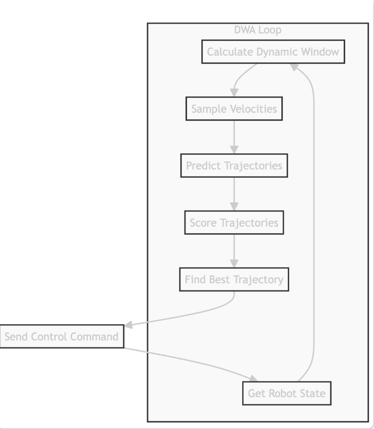
DWA Loop Steps

Calculate Dynamic Window
Sample Velocities
Predict Trajectories
Score Trajectories
Find Best Trajectory
Send Control Command
Get Robot State

Each trajectory is simulated for a short time (dt = 0.1s), and the best trajectory is chosen to control the robot.

Notes

For every showed path, there are fixed parameters $v \& \omega$ are fixed, and the displayed path are predicted for 3 seconds. However, in the actual process, only the first 0.1 second of the path is followed, than the robot immediately proceeds to update the predictions.

Construct Code Step by Step

python

import math 
import numpy as np
import matplotlib.pyplot as plt 
from enum import Enum

class RobotType(Enum):
    circle = 0
    rectangle = 1
    
class Config:
    """
    All simulation pararmeters 
    """
    def __init__(self):
        self.max_speed = 1.0
        self.min_speed = -1.0
        self.max_yaw_rate = 40.0 * math.pi / 180.0
        self.max_accel = 0.2
        self.max_delta_yaw_rate = 40.0 * math.pi / 180.0
        self.dt = 0.1 #time tick for motion prediction 
        self.predict_time = 3 #predict time for motion prediction (forward simulation time)
        self.v_resolution = 0.01
        self.yaw_rate_resolution = 0.1 * math.pi / 180.0
        
        self.robot_type = RobotType.circle
        self.robot_radius = 1.0
        
        #Cost Function 
        self.to_goal_cost_gain = 0.15
        self.speed_cost_gain = 1.0
        self.obstacle_cost_gain = 1.0
        self.robot_stuck_flag_cons = 0.05 # A threshold to check if the robot is stuck
        
        #Obstacle list 
        self.ob = np.array([
            [4, 4],
            [4,5],
            [4, 6],
            [5, 4],
            [5, 5],
            [5, 6],
            [6, 4],
            [6, 5],
            [6, 6]
        ])
            

def motion(state, control_input, dt):
    """

    Args:
        state: [x, y, yaw, v, w]
        control_input: [v, w]
        dt: time tick
    """
    state[2] += control_input[1] * dt
    state[0] += control_input[0] * math.cos(state[2]) * dt
    state[1] += control_input[0] * math.sin(state[2]) * dt    
    state[3] = control_input[0]
    state[4] = control_input[1]
    
    return state

def predict_trajectory(state, v, w, config):
    """
    Predict the trajectory of the robot
    """
    current_state = state.copy()
    trajectory = np.array(current_state)
    
    time = 0 
    while time <= config.predict_time:
        current_state = motion(current_state, [v, w], config.dt)
        trajectory = np.vstack((trajectory, current_state))
        time += config.dt
        
    return trajectory

def calc_to_goal_cost(trajectory, goal):
    """
    Cost of heading towards a trajectory.
    """
    # Final state of the trajectory
    final_state = trajectory[-1] 
    #trajectory[-1] is a Python trick to get the very last item from a list or array.
    
    # Angle 
    dx = goal[0] - final_state[0]
    dy = goal[1] - final_state[1]
    angle_to_goal = math.atan2(dy, dx)
    
    # Angle difference 
    heading_error = angle_to_goal - final_state[2]
    
    cost = abs(heading_error) #absolute value as we only care about the magnitude of the difference
    
    return cost

def calc_obstacle_cost(trajectory, obstacles, config):
    """
    Cost of obstacle proximity.
    """
    min_dist = float("inf") 

    # For every point in the trajectory
    for point in trajectory:
        # For every obstacle
        for obs in obstacles:
            
            dist = math.hypot(point[0] - obs[0], point[1] - obs[1])

            if dist <= config.robot_radius:
                return float("inf") 

            if min_dist > dist:
                min_dist = dist
                
    return 1.0 / min_dist

def calc_speed_cost(trajectory, config):
    """
    Speed cost
    faster = better 
    """
    final_speed = trajectory[-1, 3] # Final linear velocity
    cost = config.max_speed - final_speed
    return cost

def dwa_planner(state, config, goal, obstacles):
    """
    Dynamic Window Approach planner
    """
    dw = calc_dynamic_window(state, config)
    
    min_cost = float("inf")
    best_control_input = np.array([0.0, 0.0])
    best_trajectory = np.array(state)

    for v in np.arange(dw[0], dw[1], config.v_resolution):
        for w in np.arange(dw[2], dw[3], config.yaw_rate_resolution):

            # Predict the trajectory for this (v, w)
            trajectory = predict_trajectory(state, v, w, config)
            
            # Calculate the cost 
            goal_cost = config.to_goal_cost_gain * calc_to_goal_cost(trajectory, goal)
            speed_cost = config.speed_cost_gain * calc_speed_cost(trajectory, config)
            obstacle_cost = config.obstacle_cost_gain * calc_obstacle_cost(trajectory, obstacles, config)
            
            #Sum the costs
            final_cost = goal_cost + speed_cost + obstacle_cost

            if min_cost > final_cost:
                min_cost = final_cost
                best_control_input = np.array([v, w])
                best_trajectory = trajectory
                
    if abs(best_control_input[0]) < config.robot_stuck_flag_cons and abs(state[3]) < config.robot_stuck_flag_cons: 
        #both control and current v < the threshold, validating that the robot has stopped
        best_control_input[1] = -config.max_yaw_rate / 2.0 # Turn right
                
    return best_control_input, best_trajectory


def calc_dynamic_window(state, config):
    """
    Calculates the dynamic window
    """
    # Window from robot's absolute limits
    # [min_v, max_v, min_w, max_w]
    Vs = [config.min_speed, config.max_speed,
          -config.max_yaw_rate, config.max_yaw_rate]

    # Window from acceleration limits
    # [min_v, max_v, min_w, max_w]
    Vd = [state[3] - config.max_accel * config.dt,
          state[3] + config.max_accel * config.dt,
          state[4] - config.max_delta_yaw_rate * config.dt,
          state[4] + config.max_delta_yaw_rate * config.dt]

    # The final dynamic window is the intersection of the two
    dw = [max(Vs[0], Vd[0]),  # min_v
          min(Vs[1], Vd[1]),  # max_v
          max(Vs[2], Vd[2]),  # min_w
          min(Vs[3], Vd[3])]  # max_w
          
    return dw
            
        
def main():
    """
    Run DWA Simulation
    """
    print("sim start")
    
    config = Config()
    
    robot_state = np.array([0.0, 0.0, math.pi / 8.0, 0.0, 0.0])
    
    goal_position = np.array([10.0, 10.0])
    
    show_animation = True

    while True:
        control_input, predicted_trajectory = dwa_planner(robot_state, config, goal_position, config.ob)        # Update the robot's state by calling the motion function
        robot_state = motion(robot_state, control_input, config.dt)

        if show_animation:
            plt.cla() 
            
            plt.plot(goal_position[0], goal_position[1], "xb")
            
            plt.plot(predicted_trajectory[:, 0], predicted_trajectory[:, 1], "-g")

            plt.plot(config.ob[:, 0], config.ob[:, 1], "ok")
            
            plt.plot(robot_state[0], robot_state[1], "xr")
            
            plt.axis("equal")
            plt.grid(True) 
            
            plt.pause(0.001)
    
if __name__ == "__main__":
    main()

Time-Elastic Band (TEB)

A Time-Elastic Band (TEB) is an advanced technique used in robotics for motion planning, particularly when a robot needs to generate a smooth, collision-free trajectory while considering both spatial and temporal constraints. The method models the trajectory as a series of control points in both space and time and adjusts them to minimize a cost function. This optimization process leads to an efficient and smooth path while adhering to dynamic constraints like speed and acceleration limits.

TEB Overview

1. Trajectory Representation

The trajectory is represented by a sequence of control points $\mathbf{x}_i = (x_i, y_i, z_i, \theta_i, t_i)$ , where:

$(x_i, y_i, z_i)$ are the spatial coordinates of the control point $i$ ,
$\theta_i$ is the robot's orientation at point $i$ ,
$t_i$ is the time at which the robot reaches control point $i$ . Thus, each control point in the time-elastic band has both a spatial position and a time stamp.

2. Cost Function

The goal of the TEB approach is to optimize the trajectory by minimizing a cost function $C$ . This cost function is a weighted sum of various terms that penalize deviations from the optimal path, timing irregularities, dynamic constraints, and collisions with obstacles. The cost function is given by:

C = C_{\text{spatial}} + C_{\text{time}} + C_{\text{dynamic}} + C_{\text{collision}}

Where:

$C_{\text{spatial}}$ penalizes deviations from the planned spatial trajectory (smoothness),
$C_{\text{time}}$ penalizes irregular timing between control points,
$C_{\text{dynamic}}$ penalizes violations of dynamic constraints (e.g., velocity, acceleration),
$C_{\text{collision}}$ penalizes proximity to obstacles.

3. Spatial Cost Term $C_{\text{spatial}}$

The spatial cost term ensures the robot's path is smooth and avoids sharp deviations. It is represented by the sum of squared distances between consecutive control points:

C_{\text{spatial}} = \sum_{i=1}^{N-1} \|\mathbf{x}_i - \mathbf{x}_{i+1}\|^2

Where $\|\mathbf{x}_i - \mathbf{x}_{i+1}\|$ is the Euclidean distance between two consecutive control points, and $N$ is the total number of control points.

4. Time Cost Term $C_{\text{time}}$

The time cost term ensures that the time intervals between consecutive control points are appropriate. It penalizes large or small gaps between control points, helping to balance the timing of the trajectory. It is given by:

C_{\text{time}} = \sum_{i=1}^{N-1} (t_{i+1} - t_i)^2

Where $t_{i+1}$ and $t_i$ are the time stamps of consecutive control points.

5. Dynamic Cost Term $C_{\text{dynamic}}$

The dynamic cost term ensures that the robot adheres to its physical constraints, such as velocity and acceleration limits. This term is divided into velocity and acceleration components.

Velocity Constraints

The velocity cost term ensures that the robot does not exceed its maximum velocity $V_{\text{max}}$ . It is expressed as:

C_{\text{velocity}} = \sum_{i=1}^{N-1} \max(0, |\dot{x}_i| - V_{\text{max}})^2

Where $\dot{x}_i$ is the velocity between consecutive control points:

\dot{x}_i = \frac{x_{i+1} - x_i}{t_{i+1} - t_i}

Acceleration Constraints

The acceleration cost term ensures that the robot's acceleration does not exceed a maximum allowed acceleration $A_{\text{max}}$ . It is given by:

C_{\text{acceleration}} = \sum_{i=1}^{N-2} \max(0, |\ddot{x}_i| - A_{\text{max}})^2

Where $\ddot{x}_i$ is the acceleration between consecutive control points:

\ddot{x}_i = \frac{\dot{x}_{i+1} - \dot{x}_i}{t_{i+1} - t_i}

Thus, the total dynamic cost term is:

C_{\text{dynamic}} = C_{\text{velocity}} + C_{\text{acceleration}}

6. Collision Cost Term $C_{\text{collision}}$

The collision cost term ensures that the robot avoids obstacles by penalizing proximity to them. It is defined as:

C_{\text{collision}} = \sum_{i=1}^{N} \max(0, d_{\text{min}} - d(\mathbf{x}_i))^2

Where:

$d(\mathbf{x}_i)$ is the distance from the control point $\mathbf{x}_i$ to the nearest obstacle,
$d_{\text{min}}$ is a safety threshold distance.

This term prevents the trajectory from getting too close to obstacles by pushing the control points away from them.

7. Optimization Process

The optimization process in TEB involves adjusting both the spatial positions and the time stamps of the control points to minimize the total cost function $C$ . The optimization problem is formulated as:

\mathbf{x}_i^* = \arg\min_{\mathbf{x}_i} C(\mathbf{x}_i)

arg min means to minimize a function; whereas arg max maximizes the function

Where $\mathbf{x}_i^*$ represents the optimized control points after the optimization process. Typically, gradient-based optimization techniques such as gradient descent or sequential quadratic programming (SQP) are used to iteratively adjust the positions and timings of the control points.

8. Final Trajectory

After the optimization converges, the final trajectory is the path defined by the sequence of optimized control points. This trajectory is smooth, collision-free, and adheres to the robot's dynamic constraints (e.g., velocity and acceleration limits).

Conclusion:

The Time-Elastic Band (TEB) is a robust approach for motion planning in robotics, ensuring smooth, efficient, and collision-free trajectories. By minimizing a comprehensive cost function that includes spatial, temporal, dynamic, and collision-related terms, TEB optimizes the robot's path while adhering to its physical limitations. This makes TEB especially useful for robots operating in dynamic and complex environments.

Code Implementation

python

import numpy as np
import matplotlib.pyplot as plt
import matplotlib.patches as patches

class TebConfig:
    """
    Configuration class for the TEB planner.
    This holds all the parameters that define the robot's capabilities and
    the desired behavior of the optimization.
    """
    def __init__(self):
        # --- Robot Parameters ---
        self.max_velocity = 1.0  # m/s
        self.max_acceleration = 0.5  # m/s^2
        self.max_turn_rate = 0.8  # rad/s

        # --- Path and Optimization Parameters ---
        self.num_path_points = 30  # Number of points in the elastic band
        self.num_iterations = 150  # Optimization steps
        self.learning_rate = 0.05  # How much the path changes in each step

        # --- Goal Tolerance ---
        # The planner is successful if the last point is within this distance of the goal
        self.goal_tolerance = 0.2  # meters

        # --- Obstacle Parameters ---
        self.obstacle_radius = 0.5  # m
        self.min_obstacle_dist = 0.8  # Min distance to keep from obstacles (m)
        
        # --- Cost Function Weights (Gains) ---
        # These "gains" control the robot's priorities.
        self.w_obstacle = 10.0      # Weight for obstacle avoidance cost
        self.w_path_time = 1.0     # Weight for minimizing total travel time
        self.w_kinematics = 5.0    # Weight for enforcing kinematic feasibility
        self.w_velocity = 2.0      # Weight for penalizing velocity violations
        self.w_acceleration = 1.0  # Weight for penalizing acceleration violations

class TebPlanner:
    """
    A more complete implementation of the Timed Elastic Band (TEB) planner.
    """
    def __init__(self, config, start_pose, goal_pose, obstacles):
        self.config = config
        self.start = start_pose
        self.goal = goal_pose
        self.obstacles = obstacles
        
        # --- State Representation ---
        # The path is an array of (N x 4), where each row is a "pose"
        # [x, y, theta, delta_t]
        # x, y: Position
        # theta: Orientation (yaw) in radians
        # delta_t: Time interval to the *next* pose in the sequence
        self.path = self._initialize_path()

    def _initialize_path(self):
        """Creates an initial straight-line path from start to goal."""
        path = np.zeros((self.config.num_path_points, 4))
        
        # Linearly interpolate x and y
        path[:, 0] = np.linspace(self.start[0], self.goal[0], self.config.num_path_points)
        path[:, 1] = np.linspace(self.start[1], self.goal[1], self.config.num_path_points)
        
        # Calculate initial orientation (theta) along the straight line
        dx = self.goal[0] - self.start[0]
        dy = self.goal[1] - self.start[1]
        initial_theta = np.arctan2(dy, dx)
        path[:, 2] = initial_theta
        
        # Uniformly distribute time intervals (delta_t)
        # We start with an arbitrary but reasonable guess for the total time.
        total_dist = np.linalg.norm(self.goal - self.start)
        initial_total_time = total_dist / self.config.max_velocity
        path[:, 3] = initial_total_time / (self.config.num_path_points - 1)
        path[-1, 3] = 0 # The last point has no time interval to a next point
        
        return path

    def optimize(self):
        """
        The main optimization loop that iteratively refines the path.
        """
        for i in range(self.config.num_iterations):
            # The gradient is the direction of "steepest ascent" for the cost function.
            # We want to move in the opposite direction to minimize cost.
            # We calculate a gradient for each point in the path.
            gradient = np.zeros_like(self.path)

            for j in range(1, self.config.num_path_points - 1):
                # Calculate the gradients from each cost function for point j
                grad_obstacle = self._gradient_obstacle(j)
                grad_time = self._gradient_time(j)
                grad_kinematics = self._gradient_kinematics(j)
                grad_velocity, grad_accel = self._gradient_vel_accel(j)

                # Sum the gradients, weighted by their importance (gains)
                gradient[j] += self.config.w_obstacle * grad_obstacle
                gradient[j] += self.config.w_path_time * grad_time
                gradient[j] += self.config.w_kinematics * grad_kinematics
                gradient[j] += self.config.w_velocity * grad_velocity
                gradient[j] += self.config.w_acceleration * grad_accel

            # Apply the gradient descent update to the path
            # We subtract the gradient because we want to move "downhill" on the cost surface.
            self.path -= self.config.learning_rate * gradient

            # Ensure delta_t remains positive
            self.path[:, 3] = np.maximum(0.01, self.path[:, 3])

            self.plot(i)
            
            # Check for convergence
            if np.linalg.norm(self.path[-1, 0:2] - self.goal) < self.config.goal_tolerance:
                print(f"Goal reached in {i} iterations.")
                break

    # --- Gradient Calculation Functions ---
    # These functions calculate the "push" and "pull" on the path points.

    def _gradient_obstacle(self, j):
        """Calculates the repulsive force from obstacles."""
        grad = np.zeros(4)
        pos = self.path[j, 0:2]
        
        for obs in self.obstacles:
            dist_vec = pos - obs
            dist = np.linalg.norm(dist_vec)
            
            if dist < self.config.min_obstacle_dist:
                # This gradient pushes the (x, y) coordinates of the point
                # directly away from the obstacle. The push is stronger when closer.
                grad[0:2] += (dist_vec / dist) * (1 - dist / self.config.min_obstacle_dist)
        return grad

    def _gradient_time(self, j):
        """This gradient encourages shrinking the time intervals (delta_t) to create faster paths."""
        grad = np.zeros(4)
        # The gradient for the cost function `Cost = dt` with respect to `dt` is 1.
        # This creates a constant "pull" to make delta_t smaller.
        grad[3] = 1.0
        return grad
        
    def _gradient_kinematics(self, j):
        """Ensures the robot's orientation (theta) aligns with its direction of travel."""
        grad = np.zeros(4)
        pos_prev, pos_curr, pos_next = self.path[j-1, 0:2], self.path[j, 0:2], self.path[j+1, 0:2]
        theta = self.path[j, 2]
        
        # The direction the robot is *actually* traveling
        path_direction_vec = pos_next - pos_prev
        path_angle = np.arctan2(path_direction_vec[1], path_direction_vec[0])
        
        # The difference between where the robot is pointing and where it's going
        angle_diff = path_angle - theta
        # Normalize the angle difference to be within [-pi, pi]
        angle_diff = (angle_diff + np.pi) % (2 * np.pi) - np.pi
        
        # This gradient pushes the theta of the point to align with the path direction.
        grad[2] = angle_diff
        return grad

    def _gradient_vel_accel(self, j):
        """Penalizes violations of velocity and acceleration limits."""
        grad_vel = np.zeros(4)
        grad_accel = np.zeros(4)

        # Get relevant poses and time intervals
        p_prev, p_curr, p_next = self.path[j-1], self.path[j], self.path[j+1]
        dt_prev, dt_curr = p_prev[3], p_curr[3]

        # --- Velocity ---
        v_curr = (p_curr[0:2] - p_prev[0:2]) / dt_prev
        vel_mag = np.linalg.norm(v_curr)
        if vel_mag > self.config.max_velocity:
            # If velocity is too high, the gradient pushes to *increase* the
            # time interval (dt) of the *previous* segment to slow down.
            grad_vel[3] = 2 * (vel_mag - self.config.max_velocity)

        # --- Acceleration ---
        if j > 1:
            p_prev2 = self.path[j-2]
            dt_prev2 = p_prev2[3]
            v_prev = (p_prev[0:2] - p_prev2[0:2]) / dt_prev2
            
            accel = (v_curr - v_prev) / dt_prev
            accel_mag = np.linalg.norm(accel)
            if accel_mag > self.config.max_acceleration:
                # If acceleration is too high, this gradient pushes to increase
                # the time intervals of the surrounding segments to smooth the motion.
                grad_accel[3] = 2 * (accel_mag - self.config.max_acceleration)

        return grad_vel, grad_accel
        
    def plot(self, iteration):
        """Visualizes the current state of the planner."""
        plt.cla()
        # Plot Path
        plt.plot(self.path[:, 0], self.path[:, 1], 'g-', label="Elastic Band")
        
        # Plot Robot Poses (Position and Orientation)
        for i in range(self.config.num_path_points):
            pos = self.path[i, 0:2]
            theta = self.path[i, 2]
            plt.arrow(pos[0], pos[1], 0.2 * np.cos(theta), 0.2 * np.sin(theta),
                      head_width=0.1, color='b')

        # Plot Obstacles
        for obs in self.obstacles:
            circle = patches.Circle(obs, self.config.obstacle_radius, color='r', fill=True)
            plt.gca().add_patch(circle)

        # Plot Start and Goal
        plt.plot(self.start[0], self.start[1], 'bs', markersize=10, label="Start")
        plt.plot(self.goal[0], self.goal[1], 'y*', markersize=15, label="Goal")

        plt.title(f"TEB Optimization - Iteration: {iteration}")
        plt.xlabel("X Position (m)")
        plt.ylabel("Y Position (m)")
        plt.axis("equal")
        plt.grid(True)
        plt.legend()
        plt.pause(0.01)

def main():
    """Main function to set up and run the TEB planner."""
    print("Advanced TEB demonstration start!")
    
    config = TebConfig()
    start_pose = np.array([0.0, 0.0])
    goal_pose = np.array([12.0, 12.0])
    obstacles = [
        np.array([4.0, 3.0]),
        np.array([5.0, 6.0]),
        np.array([8.0, 9.0]),
        np.array([9.0, 7.0])
    ]
    
    planner = TebPlanner(config, start_pose, goal_pose, obstacles)
    planner.optimize()
    
    print("TEB optimization finished.")
    plt.show()

if __name__ == '__main__':
    main() 

Dynamic Window Approach (DWA) Planner

What is the "Dynamic Window"?

1. Searching Space

2. Optimization

3 Key Questions

Constraints

Dynamic Window

DWA Loop Steps

Notes

Construct Code Step by Step

Time-Elastic Band (TEB)

1. Trajectory Representation

2. Cost Function

3. Spatial Cost Term CspatialC_{\text{spatial}}Cspatial​

4. Time Cost Term CtimeC_{\text{time}}Ctime​

5. Dynamic Cost Term CdynamicC_{\text{dynamic}}Cdynamic​

Velocity Constraints

Acceleration Constraints

6. Collision Cost Term CcollisionC_{\text{collision}}Ccollision​

7. Optimization Process

8. Final Trajectory

Conclusion:

Code Implementation

3. Spatial Cost Term $C_{\text{spatial}}$

4. Time Cost Term $C_{\text{time}}$

5. Dynamic Cost Term $C_{\text{dynamic}}$

6. Collision Cost Term $C_{\text{collision}}$